Ordinary magnetoresistance of Cu

In this note, we are going to use WannierTools to study the ordinary magnetoresistance of Cu. More details of the results can be found in this paper Shengnan Zhang, Quansheng Wu, Yi Liu, Oleg V. Yazyev PhysRevB.99.035142, (2019). DOI:10.1103/PhysRevB.99.035142. arXiv:1808.08178

Relevant files of this example are included in directory wannier_tools/examples/Cu. In this example, we are going to study the ordinary magnetoresistance of Cu when the applied field is along the z-direction.

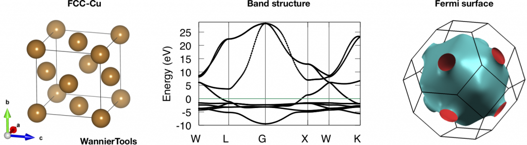
1. First, let’s calculate the band structure and the Fermi surface.
$ cp wt.in-bands wt.in
$ mpirun -np 4 wt.x

Use gnuplot to plot the band structure.

$ gnuplot bulkek.gnu

Use Xcrysden to visualize the Fermi surface

$ xcrysden –bxsf FS3D.bxsf

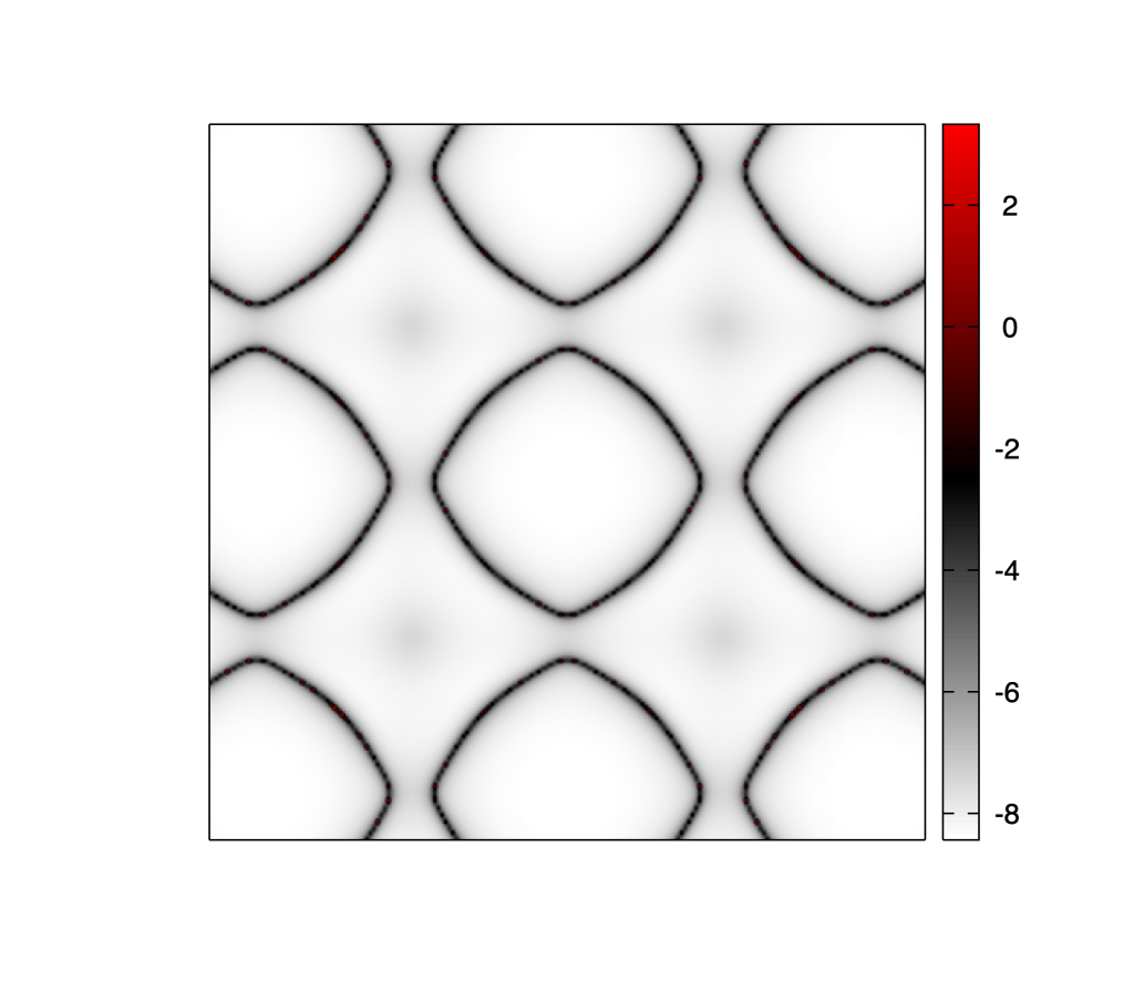
Fig. 1. Crystal structure, band structure, Fermi surface of FCC Cu

2. Then we can try to analyze the Fermi surface cross-section that perpendicular to the magnetic field. For example, we can study the Fermi surface cross-section at the $k_z$ =0 plane.

$ cp wt.in-FS-contour wt.in
$ mpirun -np 4 wt.x

Obtain the fs_kplane.png with fs_kplane.gnu.

$ gnuplot fs_kplane.gnu

You can also modify the KPLANE_BULK section to get other cross-sections as shown in Fig 5 of PhysRevB.99.035142 .

Fig 2. Fermi surface cross-section of Cu at kz=0.

3. Use Boltz_OHE_calc=T to get the ordinary magnetoresistance. The illustration of the parameters is shown here. Here we prepared four input files for different magnetic field directions Btheta=0, 18, 30, 45 degrees.

$ cp wt.in-OHE-theta0 wt.in

mpiexec -np 4 wt.x &

cp rho_band_6_mu_0.00eV_T_30.00K.dat rho_band_6_mu_0.00eV_T_30.00K.dat-theta0

$ cp wt.in-OHE-theta18 wt.in

mpiexec -np 4 wt.x &

cp rho_band_6_mu_0.00eV_T_30.00K.dat rho_band_6_mu_0.00eV_T_30.00K.dat-theta18

$ cp wt.in-OHE-theta30 wt.in

mpiexec -np 4 wt.x &

cp rho_band_6_mu_0.00eV_T_30.00K.dat rho_band_6_mu_0.00eV_T_30.00K.dat-theta30

$ cp wt.in-OHE-theta45 wt.in

mpiexec -np 4 wt.x &

cp rho_band_6_mu_0.00eV_T_30.00K.dat rho_band_6_mu_0.00eV_T_30.00K.dat-theta45

And we prepared one script to plot the $\rho_{xx}$ .

$ gnuplot rho.gnu

The generated file rho.pdf should look like Fig 4 (d) of PhysRevB.99.035142.

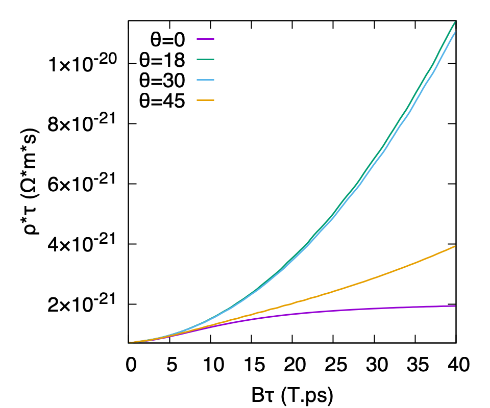
Fig 3. Magnetoresistance from Fermi surface topology
Resistivity $\rho_{xx}$ as a function of the magnitude of magnetic field B for the four field directions with $\theta=0,18, 30, 45$ degree, $\phi=90$ .

Notes:

In this example, there is only one band crossing the Fermi level. So we can just use the resistivity files. However, if you have several bands, you have to write a script sum up all the sigma files belong to the same band, same temperature and same chemical potential, then inverse the matrix to get the resistivity tensor.
In the sigma file, WannierTools write out the $\sigma_n/\tau_n$ instead of $\sigma_n$ . So when you do the summation of the $\sigma_n$ , you should set $\tau_n$ for each band first. $\tau_n$ could be different for different bands. This is one freedom for users. Different materials could have different behaviors.